
EMAP2SEC
Emap2sec identifies the secondary structures of proteins in cryo-EM maps of intermediate resolution range (~5 to 10 Å) .
Emap2sec uses convolutional deep neural network as its core algorithm and assigns a secondary structure to each of the grid points in an EM map
Introduction
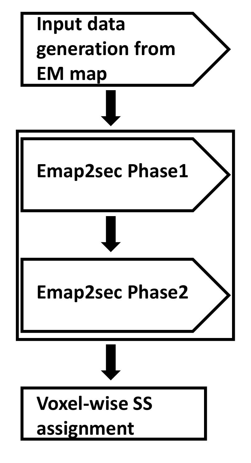
Emap2sec architecture has 4 main steps:
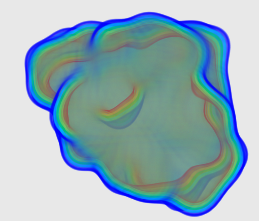
(1) Data generation from an input EM map - This step takes in your EM map and formats the map file into an input file for Emap2sec.
(2) Emap2sec phase1 - This is the first phase of our deep learning model consisting of a convolutional neural network (CNN) for local structure detection.
(3) Emap2sec phase2 - This is the second step of our deep learning model and it essentially performs prediction smoothing to eliminate obvious false positives and false negatives.
(4) Voxel-wise secondary structure (SS) assignment - The final step that gives out secondary structure assignments for your EM map.
Tutorial
Architecture
The architecture of Emap2sec is summarized in the flowchart on the right.
This document will provide a detailed explanation of each step of the Emap2sec architecture and programs needed to run those steps. It concludes by giving a step-by-step application walk-through on a simulated and an experimental EM map.
Input file generation from your EM map
The input file for Emap2sec is generated in two-steps. In the first step, a program named map2train_fix takes an EM map and relevant details such as the map's author recommended contour level and pixels/Angstrom values as input and generates an intermediate readable text file called [your_map_id]_trimmap. A trimmap contains normalized electron density values of voxels. In the second step, a program named dataset uses this trimmap to generate an input file called [your_map_id]_dataset, which contains rows of density values that we get by scanning the input map in all the 3 directions using a 11*11*11 cube. Emap2sec makes secondary structure assignment to each of these rows.
Emap2sec phase1 - CNN for local structure detection
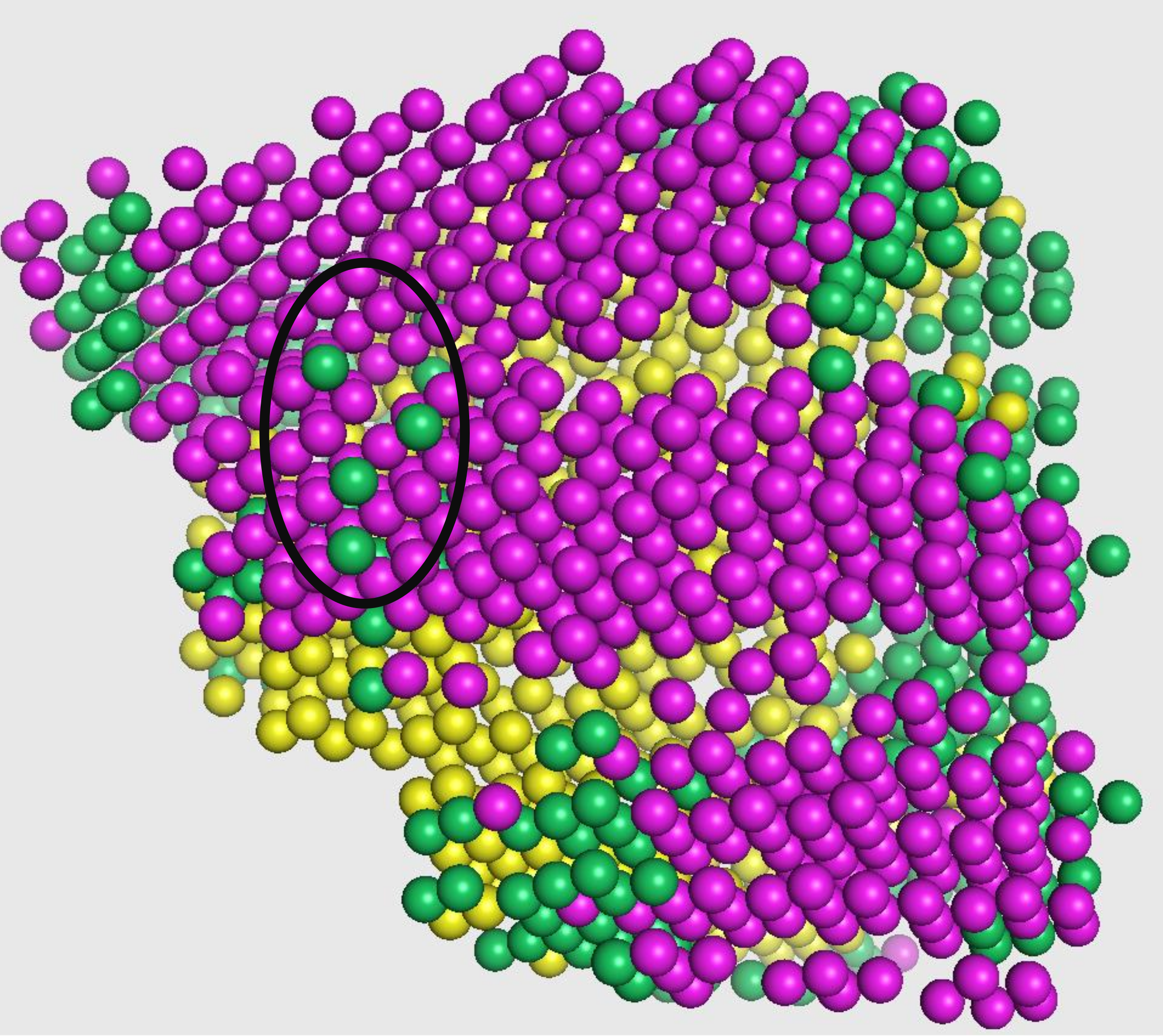
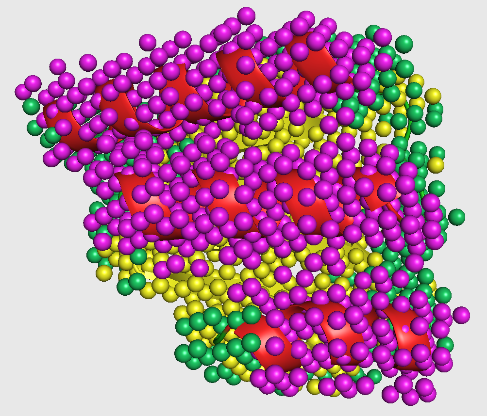
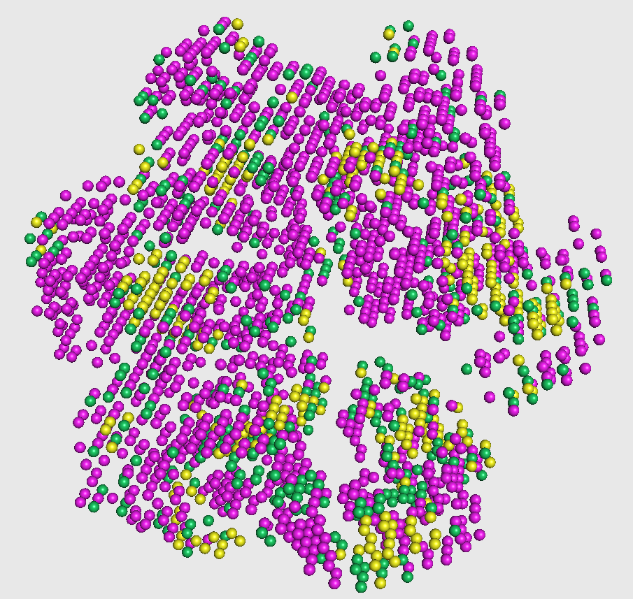
The test dataset generated in the previous step is fed to the first phase of Emap2sec that contains a convolutional neural network (CNN). This step gives out probability values of helix, sheet, and other for each cube.
In the figure, magenta spheres correspond to helix predictions, yellow spheres correspond to sheet predictions, and green spheres correspond to other (coil/turn) predictions.
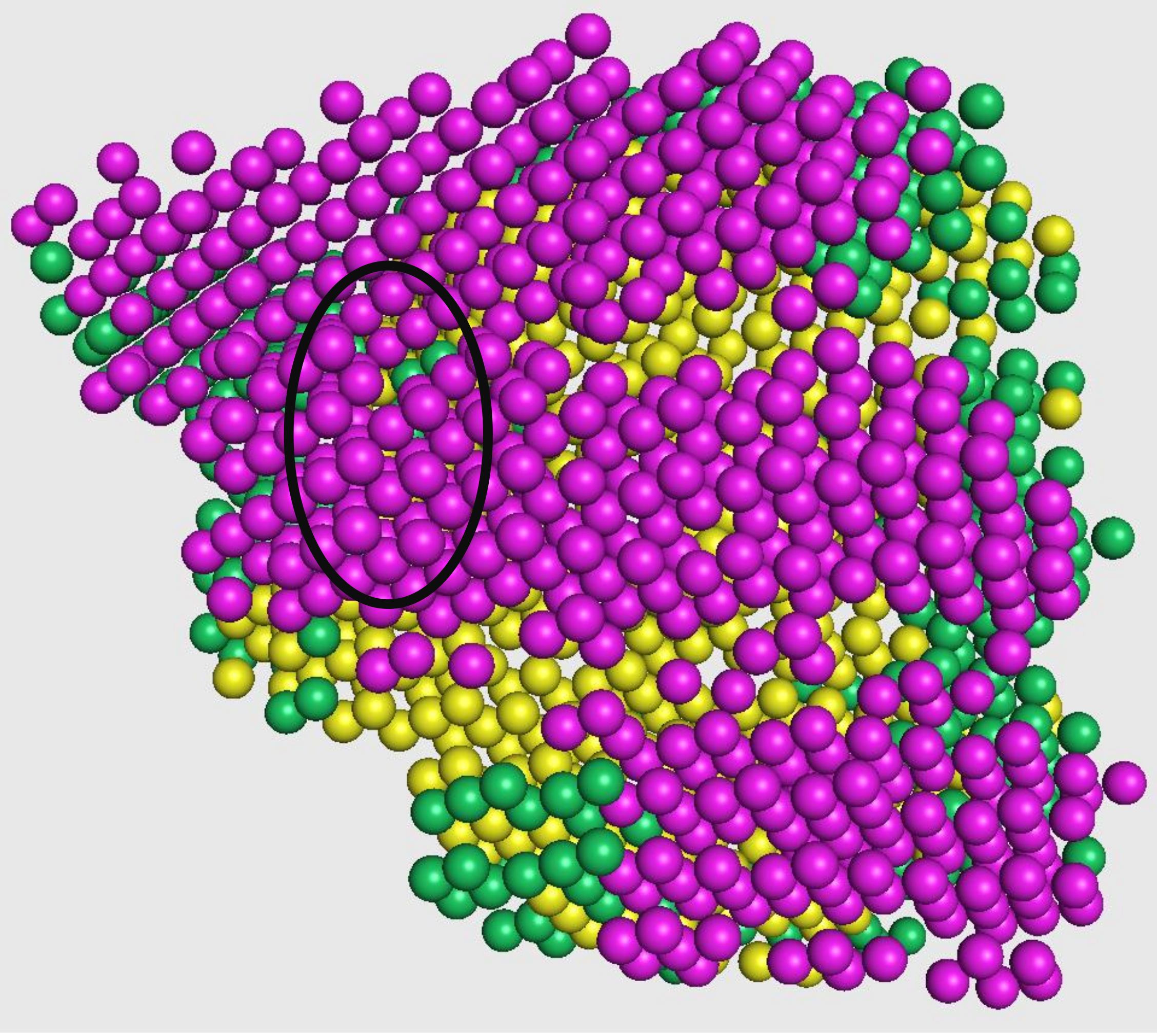
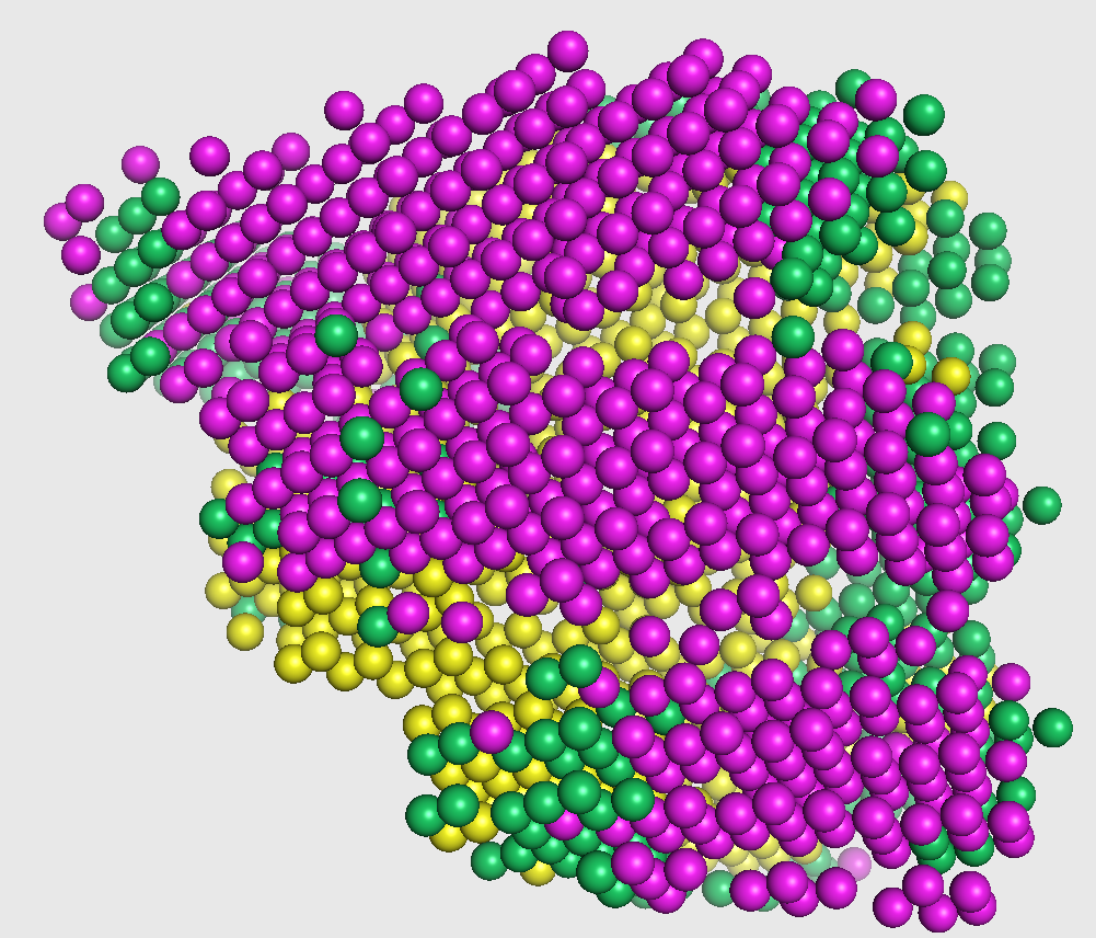
Emap2sec phase2 - Prediction smoothing
The output from the first phase is a set of predicted probabilities for each of helix, sheet, and other structures. In this second phase, these probabilities are used to smooth out any infeasible predictions given in the first phase (such as having an isolated coil in the middle of helices, as highlighted in the figure on the right).
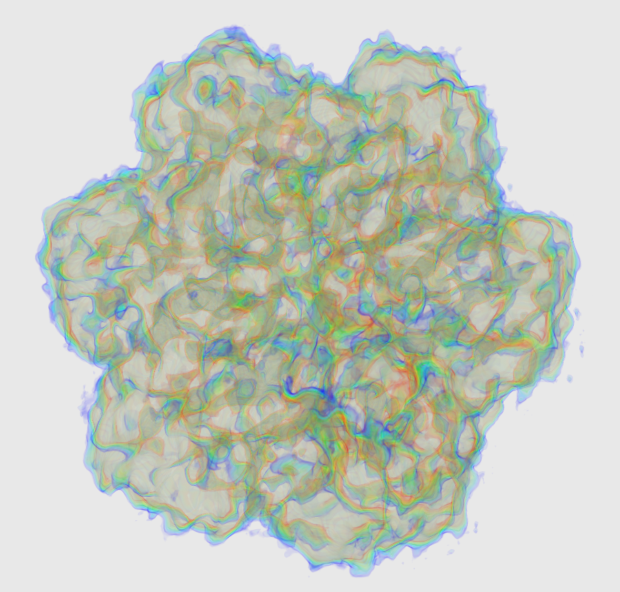
Voxel-wise SS assignment
The final voxel-wise secondary structure assignment for the cryo-EM map is done using the output class labels from phase 2.
In the figure on the right, we superimpose our assignments on the underlying crystal structure.
Usage guide
In the following section, we give a step-by-step guide to run various programs that we talked about in the earlier section. You can find the link for these programs in Downloads tab.
Input file generation
Generate the input file called [your_map_id]_dataset from your map file by following these 3 steps.
1) Trimmap File generation
        data_generate/map2train_fix [sample_mrc] [options] > [output_trimmap_filename]

        INPUTS:

        map2train_fix expects sample_mrc to be a valid filename. Supported file formats are Situs, CCP4, and MRC2000.
        Input may be gzipped. Format is deduced from FILE's extension.


        OPTIONS:(Options marked with asterisk (*) are to be used only for benchmark purposes i.e., when you've the
          underlying crystal structure available)

          -c, --contour The level of isosurface to generate density values for.
          You can use a value of 0 for simulated maps and the author recommended contour level for experimental EM maps.
          default=0.0

          -g, --gzip Set this option to force reading input as gzipped.
          You can use gzip to compress a very large EM map and input the compressed file by setting this option.


          -P* PDBFILE Input a PDB file to use C-Alpha (CA) atom position.

          -r* [float] This option assigns true secondary structures labels to the generated voxels with the closest CA
          atom that's within a sphere of radius r.
          These true labels can be compared to the secondary structures assigned by Emap2sec for benchmarking.
          default=3.0

          -sstep [integer] This option sets the stride size of the sliding cube used for input data generation.
          We recommend using a value of 2 that slides the cube by 2Å in each direction.
          Decreasing this value to 1 produces 8 times more data (increase by a factor of 2 in each direction)
          and thus slows the running time down by 8 times so please be mindful lowering this value.
          default=2

          -vw [integer] This option sets the dimensions of sliding cube used for input data generation.
          The size of the cube is calculated as 2*vw+1.
          We recommend using a value of 5 for this option that generates input cube of size 11*11*11.
          Please be mindful while increasing this option as it increases the portion of an EM map a single cube covers.
          Increasing this value also increases running time.
          default=5 (->11x11x11)

          -gnorm  Set this option to normalize density values of the sliding cube, used for input data generation,
          by global maximum density value. Set this option as -gnorm.
          default=true

          -lnorm  Set this option to normalize density values of the sliding cube, used for input data generation,
          by local maximum density value. Set this option as -lnorm.
          We recommend using -gnorm option.
          default=false

          -h, --help, -?, /? Displays the list of above options.


          USAGE:
          ./map2train_fix protein.situs -c 2.75 >  protein_trimmap

          ./map2train_fix protein.map -sstep 2 -r 3.0 -c 0.0 >  protein_trimmap
2) [OPTIONAL] STRIDE File generation
Use this step to generate STRIDE file in case you have a solved crystal structure for your map. This step is for verification purposes only.
STRIDE is a secondary structure assignment program that takes a PDB file as input. You can download STRIDE from here.
      ./stride -f[output_stride_filename] [sample_pdb]


      INPUT:
      Specify the name of your pdb file in place of [sample_pdb].


      OUTPUT:
      Specify a name for output STRIDE file after -f option without space.


      USAGE:
      ./stride -fprotein.stride protein.pdb
3) Input dataset file generation
This program is used to generate input dataset file from the trimmap file generated in step 1.
This program is a python script and it works with both python2 and python3. They can be downloaded here.
STRIDE file is an optional input for this program. Provide it for benchmarking purposes only.
      python data_generate/dataset.py [sample_trimmap] {sample_stride} [input_dataset_file] [ID]


      INPUTS:
      Inputs to this script are trimmap, an optional STRIDE file, and ID is a unique identifier of a map such as
      SCOPe ID, EMID, etc.


      OUTPUT:
      Specify a name for input dataset file in place of [input_dataset_file].


      USAGE:
      python data_generate/dataset.py protein_trimmap protein_dataset protein_id
      python data_generate/dataset.py protein_trimmap protein.stride protein_dataset protein_id
Emap2sec SS identification (Phase1 and Phase2)
Run Emap2sec program for identification of secondary structures.
Use emap2sec/Emap2sec_sim.py when your input is a simulated EM map and use emap2sec/Emap2sec_exp.py when your input is an experimental EM map.
This program is a python script and it works with both python2 and python3.
      python emap2sec/Emap2sec_[sim/exp].py [dataset_location_file]

      INPUT:
      This program takes input as a file that contains location of input dataset.
      It also allows you to test multiple files at a time. File locations are to be "\n" delimited.


      OUTPUT:
      This program writes two output files, one for each phase, which contain output predictions along with
      the probability value for each prediction.
      Sample output files are provided in the github link in Downloads tab and are named as outputP1_0 for Phase1
      and outputP2_0 for Phase2.


      USAGE:
      First run : echo [location of protein_dataset file] > dataset_location_file to save the location of your
      protein dataset file in dataset_location_file. You can then run emap2sec/Emap2sec_[sim/exp].py as shown below.

      python emap2sec/Emap2sec.py dataset_location_file
SS Visualization
Visualize the secondary structure assignments made in the previous step using the output file of Emap2sec SS identification program. Below program generates a PDB file containing secondary structure assignments. You can visualize these pdb structures using a molecular visualization tool such as pymol
      visual/Visual2.pl [sample_trimmap] [output_file] [OPTIONS] > out_fin.pdb

      INPUT:
      This program takes as inputs, the trimmap file generated in step 1 of input file generation
      and output file of Emap2sec SS identification.
      You can visualize Phase1 or Phase2 output by using the appropriate output file.


      OPTIONS:
      -p : Show predicted data (Predicted secondary structures)
      -n : Show native data (True secondary structures)[OPTIONAL - Use in case you've the crystal structure
      information available]

      OUTPUT:
      This program outputs a pdb file that contains secondary structure assignments.
      A sample output file is provided in the github link in Downloads tab.

      USAGE:
      visual/Visual2.pl protein_trimmap outputP1_0 -p > out_fin1.pdb
      visual/Visual2.pl protein_trimmap outputP2_0 -p > out_fin2.pdb

      Upon pymol installation, from pymol download directory you can run the below code from command line,
      pymol out_fin2.pdb
      or Open Pymol GUI and load visual.pdb.

      Then run run pymol_script.py from the pymol command line. This gives you the final clean secondary structure visualization.
Examples
Simulated map example (10Å resolution)
Prepare a map file - d1kafa.mrc as an input from the PDB file d1kafa_.pdb
Generate simulated map from d1kafa_.pdb by e2pdb2mrc.py from EMAN2 package.
e2pdb2mrc.py d1kafa_.pdb d1kafa.mrc --res 10.0
Use this map file and follow the instructions in step 1 of usage guide to generate input dataset file. The trimmap file is generated as
data_generate/map2train_fix  d1kafa.mrc -r 3 -c 0
 -sstep 2 > d1kafa_trimmap
You can generate the input dataset file as follows,
python data_generate/dataset.py d1kafa_trimmap
 d1kafa_dataset d1kafa
If the generated input file is d1kafa_dataset, write the file location to a dataset location file as follows
echo ./d1kafa_dataset > test_dataset_location
Emap2sec SS identification
You can then run the Emap2sec secondary structure identification program as follows
python run_scripts/Emap2sec_sim.py test_dataset_location
Visualizing Emap2sec assignments
Two output files are generated from the previous step - outputP1_0 : output of Phase 1 and outputP2_0 : output of Phase 2.
You can visualize phase 1 output as follows
visual/Visual2.pl d1kafa_trimmap outputP1_0 -p > out_fin.pdb
and then use pymol to run
pymol out_fin.pdb
This visualization is shown in the figure captioned Phase1 assignments.
You can visualize phase 2 output as follows
visual/Visual2.pl d1kafa_trimmap outputP2_0 -p > out_fin_L2.pdb
and then run
pymol out_fin_L2.pdb
This visualization is shown in the figure captioned Phase2 assignments.

[OPTIONAL] Visualize prediction file and crystal structure together
Optionally, if you have the crystal structure available you can visualize Emap2sec final predictions
with your structure to check agreement.
The only change is before input dataset generation you generate the STRIDE file as follows,
./stride -fd1kafa.stride d1kafa_.pdb
./stride -fd1kafa.stride d1kafa_.pdb
And you generate the input dataset by specifying the STRIDE file as additional input.
python data_generate/dataset.py d1kafa_trimmap d1kafa.stride
 d1kafa_dataset d1kafa
You can then follow the same steps as earlier to generate out_fin_L2.pdb file and visualize it along with the crystal structure as follows,
pymol out_fin_L2.pdb d1kafa_.pdb
This visualization is shown in the figure captioned Crystal structure agreement.
python data_generate/dataset.py d1kafa_trimmap d1kafa.stride
d1kafa_dataset d1kafa
pymol out_fin_L2.pdb d1kafa_.pdb
Experimental map example (6Å resolution)
You can download the EM map for protein structure with EMID 8796 here. Use this map file and follow the instructions in step 1 of usage guide to generate input dataset file. The trimmap file is generated as
data_generate/map2train_fix 8796.mrc -r 3 -c 0.033 -sstep 2 \

      > 8796_trimmap
The author recommended contour level for the map EMD8796 is 0.033 which has been provided as one of the options above.
You can generate the input dataset file as follows,
python data_generate/dataset.py 8796_trimmap 8796_dataset 8796
If the generated input file is 8796_dataset, write the file location to a dataset location file as follows
echo ./8796_dataset > test_dataset_location
Emap2sec SS identification
You can then run the Emap2sec secondary structure identification program as follows
python run_scripts/Emap2sec_exp.py test_dataset_location
Visualizing Emap2sec outputs
Two output files are generated: outputP1_0 : output of Phase 1 and outputP2_0 : output of Phase 2. You can visualize phase 1 output as follows
visual/Visual2.pl 8796_trimmap outputP1_0 -p > out_fin.pdb
and then use pymol to run
pymol out_fin.pdb
This visualization is shown in the figure captioned Phase1 assignments.
You can visualize phase 2 output as follows
visual/Visual2.pl 8796_trimmap outputP2_0 -p > out_fin_L2.pdb
and then run
pymol out_fin_L2.pdb
This visualization is shown in the figure captioned Phase2 assignments.
[OPTIONAL] Visualize prediction file and crystal structure together
Optionally, if you have the crystal structure available you can visualize Emap2sec final predictions with your structure to check agreement.
The only change is before input dataset generation you generate the STRIDE file from the fitted atomic model of EMD-8796.
The pdb ID of the fitted atomic model is 5wcb and it can be downloaded here
You can generate the STRIDE file as follows,
./stride -f5wcb.stride 5wcb.pdb
./stride -f5wcb.stride 5wcb.pdb
And you generate the input dataset by specifying the STRIDE file as another input.
python data_generate/dataset.py 8796_trimmap 5wcb.stride
 8796_dataset 8796
You can then follow the same steps as earlier to generate out_fin_L2.pdb file and visualize it along with the crystal structure as follows,
python data_generate/dataset.py 8796_trimmap 5wcb.stride
8796_dataset 8796
pymol out_fin_L2.pdb 5wcb.pdb
This visualization is shown in the figure captioned Crystal structure agreement.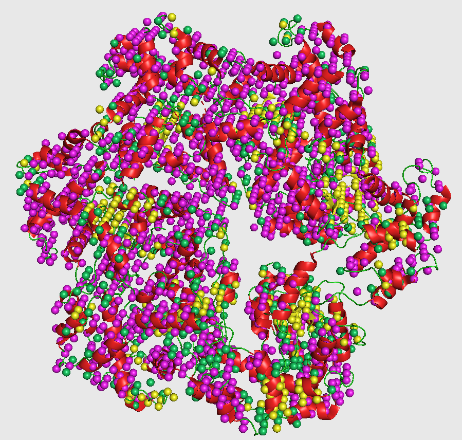
Availability
Free Server (Recommended): https://em.kiharalab.org/algorithm/emap2sec
You can run also Emap2sec on Google Colab.You can also directly run it in CodeOcean.
Full codes are available at GitHub.
Hop over to the next tab to get a detailed tutorial on how you can use our program.
Running our code ocean capsules
1. First, you need to create an account on code ocean using academic credentials and login into your account.
2. Then, click on the links above and go to the desired code ocean capsule.
3. To make a reproducible run i.e. run the code on an example input provided by us, click on the "Reproducible Run" button in the top right corner. This will start running the code on our example, and the results will be generated in the results folder at the bottom right after the execution is complete.
4. To run the code on an input of your choice, first go to our capsule and click on the "Edit Capsule" button in the top right corner. This will make a copy of our capsule which you can edit. Follow the instructions about how to upload and run your input in this copied capsule by reading the readme file present in the respective code ocean capsules.
Other details specific to the respective capsules can be found in the readme files of the capsules. For more details on how to run code ocean capsule please visit: Code Ocean user documentation
Tech Specs
CPU: >=4 cores
Memory: >=10Gb
GPU: any GPU supports CUDA with more than 12GB memory.
License
© 2018 Sai Raghavendra Maddhuri, Genki Terashi, Daisuke Kihara and Purdue University
Emap2sec is a free software for academic and non-commercial users.
It is released under the terms of the GNU General Public License Ver.3 (https://www.gnu.org/licenses/gpl-3.0.en.html).
Commercial users please contact dkihara@purdue.edu for alternate licensing.
Reference
Citation of the following reference should be included in any publication that uses data or results generated by Emap2sec program.