Introduction:

The large number of uncharacterized protein structures highlights the need for the development of computational methods for annotating proteins using the tertiary structure. These also include function annotation methods by means of characterizing protein local surfaces. In order to facilitate structure-based protein annotation, 3D-SURFER offers a web-based platform for rapid protein surface analysis and comparison. The server integrates various methods to assist in the high throughput screening and visualization of protein surface comparisons. These methods are discussed in detail below.

The new functionality for search with Alphafold models is added in October 2021.
Below, we first explain the original PDB entry search available at Search and Benchmark buttons. This section also covers a part of technical explanation for the Alphafold search page. For additional explanation for Alphafold models searches at AlphaFold, see AlphaFold Model Search section below.

Integrative Web Interface:

3D-SURFER integrates global surface shape similarity-based search using 3D Zernike Descriptors, and local structure analysis using VisGrid and LIGSITE^csc. The results obtained using these methods can be seamlessly visualized in a single intuitive user interface.

3D Zernike Descriptors :

3D Zernike Descriptors (3DZD) are utilized for the efficient comparison of protein surfaces. The descriptor is a combination of coefficients calculated from a well defined set of orthogonal 3D basis polynomials that approximate a given 3D function (a grid of a discretized surface). 3DZD has various desirable properties when applied to protein surfaces:

• Rotational invariance: Prior structural alignment is not required for protein comparisons.
• Compactness: The protein surface can be compactly represented as a feature vector with only 121 numbers (called invariants). Comparisons of these vectors can be performed by calculating Euclidean distance in very quick time, thus allowing for rapid shape retrieval.
• Hierarchical Resolution: Invariants of lower resolution are also part of the higher resolution. For example, the first 12 numbers among the 121 invariants represent the same protein at a lower resolution.

3DZD extraction procedure:

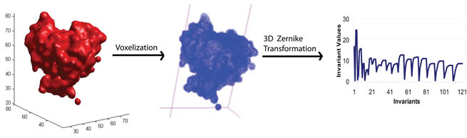
1. Voxelization: The protein surface triangulation/mesh is extracted using the MSROLL program in Molecular Surface Package version 3.9.3 [Connolly M, 1983]. The mesh is then discretized to form a cubic grid.
2. 3D Zernike transformation: The 3DZD program [Novotni M. and Klein R, 2003] takes the cubic grid as input and generates 3DZDs (the 121 invariants).

Combinatorial Extension:

• The combinatorial extension (CE) method is used to compare and align protein structures. It breaks each structure in the query set into a series of fragments that it then attempts to reassemble into a complete alignment. A series of pairwise combinations of fragments called aligned fragment pairs, or AFPs, are used to define a similarity matrix through which an optimal path is generated to identify the final alignment. Only AFPs that meet given criteria for local similarity are included in the matrix as a means of reducing the necessary search space and thereby increasing efficiency. Pairwise aligment can be performed via the web at http://cl.sdsc.edu/ce.html.

VisGrid:

• The VisGrid algorithm facilitates the characterization of local geometric features of protein surfaces in an interactive manner using various features provided by the visibility criterion. The visibility is defined as the fraction of visible directions from a target position on a protein surface. A pocket or a hollow is recognized as a cluster of positions with a small visibility. A large protrusion in a protein structure is recognized as a pocket in the negative image of the structure. While existing methods restrict themselves to locating pockets with potential ligand binding site behavior, VisGrid can also focus on the dominant geometric features in the protein structure by identifying large protrusions, hollow and flat regions on the surface.

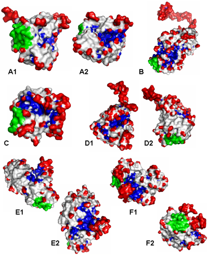
• The above figure illustrates various examples of protein surface cavities (Blue), protrusions (red), and flat regions (green) identified by the visibility criterion using VisGrid.

LIGSITE^csc:

• LIGSITE^csc is an algorithm for the automatic identification of pockets on protein surface using the Connolly surface and the degree of conservation.

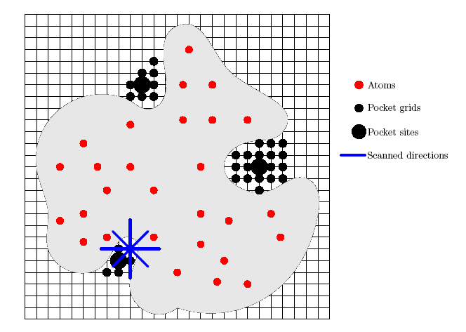
• The procedure to identify pockets is as follows: First, the protein is projected onto a 3D grid step size of 1.0 Angstrom. Second, grid points are labelled as protein, surface, or solvent. A sequence of grid points, which starts and ends with surface grid points and which has solvent grid points in between, is called a surface-solvent-surface event. LIGSITE^csc scans the x, y, z directions and four cubic diagonals for such surface-solvent-surface events. If a solvent grid point is part of at least five surface-solvent-surface events, it is marked as pocket. Finally, all pocket grid points are clustered according to their spatial proximity, i.e., if a pocket grid point is within 3.0 Angstrom to a pocket grid point cluster, it is added to this cluster. Otherwise, it becomes a new cluster. Next, the clusters are ranked by the number of grid points in the cluster. The top three clusters are retained and re-ranked according to the degree of conservation of the involved surface residues.

Query entry IDs:

The input data is a protein structure, which will be compared against a user-specified dataset of the entire PDB database. The input structure is provided by entering its identification (ID) code or by uploading a PDB format file to the server.

The ID code of an input protein structure is named based on the PDB ID of the protein. If an entire structure (e.g. a protein complex) in a PDB file is chosen for input, the ID is the same as the PDB code (e.g. 7tim). However, some subunits are clustered as separated as different entries (e.g. 12e8-C01 with Chain H, L and 12e8-C02 with Chain M, P), if the clusters are far apart from each other with a minimum distance at 4.5 Angstrom. A chain in a PDB file can be specified by adding a hyphen and the chain ID following the PDB code, e.g. 7tim-A. A domain of a chain can be specified by further adding a domain ID that is defined by CATH, (e.g. 7tim-A-01). The composition of the complex (i.e. chains in 12e8-C02) and domain (i.e. residues range) entries are shown when users move the mouse on the ids below the pictures in the resulting page.

Please click to download Chain composition of complexes and Residue id range of domains

Basic features available through 3D-SURFER:

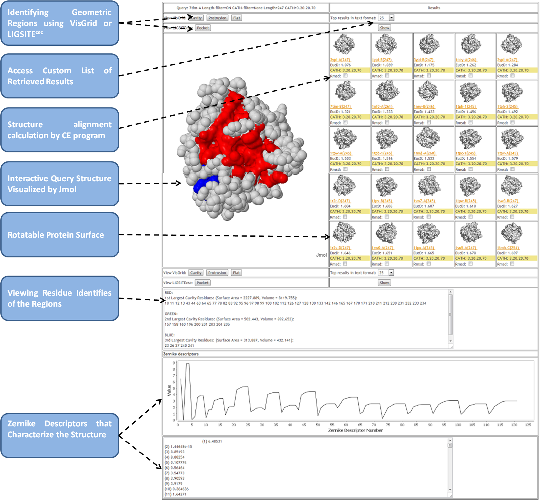
• Viewing surface comparison results
  • Comparisons are performed by calculating the Euclidean distance (the square root of the sum of the squares of the differences between corresponding values) between the Zernike feature vectors (121 scalar values) representing the proteins. In the 3D-Surfer results, this is shown after label, "EucD:" .
• Viewing surface analysis results
  • The JSmol applet can be used to rotate the query structure and color the surface by cavity, protrusion, and flatness. Clicking on the buttons called "Cavity", "Protrusion", or "Flat" will render the surface in three different colors based on their rank in terms of geometric visibility: Red (1st), Green (2nd), and Blue (3rd). Also shown are the volumes (in cubic Angstrom) and surface areas (in square Angstrom) of the convex hull formed from the atom coordinates of the residues identified by VisGrid.
• Rotatable protein surface figures
  • Protein surfaces can be rotated by moving the mouse over each of the images of the results. The images will spin 360° along both the X and Y axes to give a complete view of the protein surface.
• Structure alignment calculations and visualization
  • Structure-based alignments of the proteins can be obtained by using the Combinatorial Extension (CE) program. To execute CE, check "RMSD:" box of proteins in comparison to your query structure. If the calculation was possible, the RMSD value and the coverage (the number of aligned amino acids divided by the length of the query entry) will be displayed,and a new button will appear; if this button is clicked, the visualization of the CE alignment will appear on the left panel.
• Viewing CATH codes
  • CATH codes for each of the results can also be viewed next to the "CATH: " section.
  • If a structure does not have an assigned CATH code, it shows "N/A"
  • Currently, AF2 models do not have a CATH code.
• CATH code filtering
  • It is common that the results returned are very similar, in terms of the CATH codes they have. If the user wants, for example, to get results that are different in terms of the first two levels (specify CATH filter as "CA"), then the query will avoid returning repeated results for structures that share the first two levels. In other words, if two structures have CATH codes 3.40.390.10 and 3.40.50.300, only one of them would be returned, because 3.40 is repeated.
• Length filtering
  • When "Residue Length Filter" is enabled, the results returned will be similar in terms of the number of residues that each structure has. Two structures are considered similar if the size of one with respect to the other is between 0.57 and 1.75 times the size of the other one.
• PDB Link
  • Each reported result displays the corresponding PDB ID and is directly linked to the PDB website.
• Zernike Invariants
  • The 121 Zernike Invariants (or Zernike Descriptors), that characterize each structure are displayed in text and graphic forms, below the molecule visualization component.

Batch search and 3DZD computation on Benchmark page:

"Benchmark" page provides the option to obtain 3D-SURFER search results in a batch mode, and also compute 3DZD for all query proteins.

• Batch database search: Click on "Normal database search request" at the top of Benchmark page. In "Step 1", query proteins are provided by entering their ID codes in "Structure id list" box or by uploading a structure id list file. After choosing surface representation in "Step 2", users can click on "Get 3D Zernike Descriptor" button in "Step 3" to open 3DZD result page in a new tab.
• 3DZD computation: Click on "Compute 3DZDs for zipped PDB files" at the top of Benchmark page. In "Step 1", PDB files for proteins of interest are submitted as a single zipped file. The 3DZD calculation result will be sent to the provided email address after calculation is done. After choosing surface representation in "Step 2", users can click on "Submit" button to submit their 3DZD calculation job.

AlphaFold Model Search:

This is a new functionality of this webserver available at the "AlphaFold" tab, which incorporated computational protein models built by Alphafold2. Alphafold2 models were retrieved from AlphaFold Protein Structure Database .
From each model, To extract a confident domain in an Alphafold2 model, we first extracted all contiguous regions of more than 50 confident residues that have a pLDDT score greater than 70.0. Then, confident regions separated by at most 5 non-confident residues were merged, along with the intervening residues regardless of confidence level. AlphaFold2 models were discarded if they have no confident domains.
As of October 14, 2021, 508,787 domains are included from 21 proteomes. A search can be performed within AlphaFold2 models, or across AlphaFold2 models (AF2 models) and PDB entries.

• [Step 1] To specify the AF2 model as a query, type the first couple of letters of its AF2 model IDs and the rest will be autofilled. The ID is followed by F1, which is also associated with the PDB file of the original AF2 model, then maybe followed by two numbers, such as 1-417, if the structure is a domain extracted from the full AF2 model of the Alphafold model ID. The two numbers are the starting and ending residue positions. Then, at the end of an ID, AFv1 is attached as a suffix indicating this is a model by Alphafold version 1 as proivided in the Alphafold Database.


• [Step 2] Choose representation. Main-chain atom is more accurate for protein fold level recognition.


• [Step 3] Choose the database to search against. Complexes in PDB are not included among the databases you can choose.


• [Step 4] As in the original 3D-Surfer Search, when the length filter is on, two structures are considered similar if the size of one with respect to the other is between 0.57 and 1.75 times the size of the other one.


• [Step 5] The default choice, "3D-Surfer + Neural Network" uses deep neural network that was trained to retreive protein structures of the same SCOPe fold from their 3DZD vectors. The architecture of the network is provided in a previous work [see Reference 8]. The network was newly trained on 256,391 structures in 1,430 unique folds in SCOPe (ver. 2.07). For identifying proteins of the same fold, this option performs better than choosing original 3D-Surfer. On the other hand, 3D-Surfer will be able to identify proteins that have the same surface shapes, which often could lead to an interesting biological finding.

Documentation References:

1. Lee Sael, Bin Li, David La, Yi Fang, Karthik Ramani, Raif Rustamov and Daisuke Kihara. Fast protein tertiary structure retrieval based on global surface shape similarity. Proteins: Structure, Function, and Bioinformatics 72:1259-1273(2008).
2. Bin Li, Srinivasan Turuvekere, Manish Agrawal, David La, Karthik Ramani and Daisuke Kihara. Characterization of local geometry of protein surfaces with the Visibility Criterion. Proteins: Structure, Function, and Bioinformatics 71:670-683(2008).
3. Connolly ML. Solvent-accessible surfaces of proteins and nucleic acids. Science 1983;221(4612):709-713.
4. Novotni M, Klein R. 3D Zernike descriptors for content based shape retrieval.ACM Symposium on Solid and Physical Modeling, Proceedings of the eighth ACM symposium on Solid modeling and Applications 2003;216-225.
5. Huang B, Schroeder M. LIGSITE^csc: predicting ligand binding sites using the Connolly surface and degree of conservation.BMC Struct Biol2006;6:19.
6. Jumper J, Evans R, Pritzel A, et al. Highly accurate protein structure prediction with AlphaFold. Nature. 2021;596(7873):583-589.
7. Tunyasuvunakool K, Adler J, Wu Z, et al. Highly accurate protein structure prediction for the human proteome. Nature. 2021;596(7873):590-596.
8. Raffo, A., Fugacci, U., Biasotti, S., et al. SHREC 2021: Retrieval and classification of protein surfaces equipped with physical and chemical properties. Computers & Graphics, 99;2021;1-21.

Latest updates of 3D-SURFER:

• 2021/10/14: AlphaFold search page added.
• 2019/05/21: fix a bug in 3DZD calculation.
• 2018/11/20: add the option to calculate 3DZD for zipped PDB files on benchmark page.
• 2018/09/17: add the option to download 3D Zernike Descriptors on benchmark page.
• 2018/02/13: fix the update of CATH domains every week.
• 2018/01/10: update CATH classfication every week.
• 2017/09/18: use multiprocessing to identify contact pairs in complex pdb.
• 2017/07/17: fix a problem in updating list files.
• 2017/07/10: use multiprocessing to generate images and animations.
• 2017/06/29: zernike is replaced by map2zernike.
• 2017/06/23: update pymol-0.98/ to latest pymol-v1.8.6.2, update PDB download link, replace obj2grid with latest compiled one.
• 2017/01/01: enable the search using a web link.